Rank-Nullity, Dual Spaces, Strang’s Fundamental Subspaces (Linear Maps, pt 1)

The theory of linear maps is simple and elegant. In principle, the rules of linear algebra computation should become intuitive once the theory is understood. This knowledge will spare you from suffering in all sorts of domains; e.g., it will be easy to pick up Dirac notation in quantum mechanics, and the Riesz representation theorem will resolve any insecurity in using it.

I’ll attempt to provide a condensed summary of the theory for reference, with sketches of proofs mostly following Axler’s text. This first post will cover the fundamentals, culminating with Strang’s four fundamental subspaces. More advanced material will be covered in part two.

Vector spaces

• A group $(G,\cdot)$ is a set of objects $G$ and a binary operation $\cdot$ such that
  • $G$ is closed under $\cdot$,
  • $\cdot$ is associative,
  • there is an identity element, and
  • every element has an inverse element.
• A ring is an abelian group under addition ($+$) and a monoid under multiplication ($\cdot$) (ie $\cdot$ is associative and there exists a multiplicative identity).
  • Multiplication is distributive with respect to addition.
  • Example: $\Z$ is a commutative ring but not a field.
• A field is a commutative ring such that every nonzero element has a multiplicative inverse.
  • Can think of as a ring whose nonzero elements are an abelian group under multiplication.
  • Examples: $\Q,\R,\C$.
• A vector space is an abelian group $(V,+)$ with scalar multiplation over a field $\F$.
  • Vector addition and scalar multiplication interact via the distributive properties, and there exists a multiplicative identity.

• By definition, a finite dimensional vector space has a finite list of spanning vectors.

• A spanning list can be reduced to a basis by iterating through the list and removing vectors in the span of previously iterated vectors.

• It follows that every finite dimensional vector space has a basis.

• Every linearly independent list can be extended to a basis by appending a basis to it (which exists per above), thereby producing a spanning list; then reducing it to a basis as above.

• (Sum of subspaces.) If $U_1,U_2$ are subspaces of $V$, then $V = U_1 + U_2$ if for every $v \in V$ there exist $u_1 \in U_1$, $u_2 \in U_2$ such that $v = u_1 + u_2$.
  • The sum $V = U_1 + U_2$ is a direct sum, denoted $V = U_1 \oplus U_2$, if every $v \in V$ can be expressed uniquely as a sum $v = u_1 + u_2$.
• $U_1 + U_2$ is a direct sum if and only if $U_1 \cap U_2 = \{0\}$.
  • $\implies$: Suppose $u \in U_1 \cap U_2$. The decompositions $u = u + 0$ and $u = 0 + u$ are the same if and only if $u = 0$.

  • $\impliedby$: Suppose $u = u_1 + u_2$ and $u = w_1 + w_2$, where $u_1,w_1 \in U_1$ and $u_2,w_2 \in U_2$. Then

    \[u - u = \underbrace{(u_1 - w_1)}_{\in U_1} + \underbrace{(u_2 - w_2)}_{\in U_2} = 0.\]

    So we have

    \[u_1 - w_1 = - (u_2 - w_2)\]

    which implies $u_1 - w_1, u_2 - w_2 \in U_1 \cap U_2$. Therefore $u_1=w_1$ and $u_2 = w_2$, proving the direct sum property.

• Let $U$ be a list of linearly independent vectors and let $W$ be a spanning list. Then $\length U \leq \length W$.
  • Put the vectors $w_i$ into a list $B$. Append $u_1$ to the beginning of $B;$ this is a linearly dependent list so there is a $w_i$ that can be removed from $B$ that preserves $\span B $. You can repeat this procedure until all the $u_i$ are added, with a $w_i$ removed with each $u_i$ added, so $\length U \leq \length W $.
• Therefore, all bases of a vector space have the same length, called dimension.

Linear maps

• $\null T = \{0\} \iff T$ injective

• $\dim V = \rank T + \dim \null T $, known as the rank-nullity theorem.
  • Let $\{u_i\}$ be a basis for $\null T $. Extend it to a basis for $V;$ call the added vectors $\{v_i\}$. Then $\{T(v_i)\}$ is a basis for $\range T $.

• If $\dim V > \rank T $, then $T$ is not injective by rank-nullity.

• If $T: V \rightarrow W$, and $\dim V < \dim W$, then $T$ cannot be surjective because $\rank T $ because $\rank T \leq \dim V $ by rank-nullity.

• A system of $m$ linear equations captures the act of sending a vector of $n$ variables $\{x_i\}$ through $T: \F^n \rightarrow \F^m$, where the values of the equations is a vector in $\F^m$. If $m > N$ (more equations than variables), then there are values of the equations $\in \F^m$ for which there are no solutions $\{x_i\}$, because $\rank T \leq n < m$ by rank-nullity; i.e., $\range T \neq \F^m$.

• A system of linear equations is homogeneous if it sends $\{x_i\}$ to $0 \in \F^m$. Asking whether there are nonzero solutions is the same as asking whether $\dim \null T > 0$, which is definitely true when $m < n$ because $\rank T \leq m < n$.

• $T$ has an inverse map (i.e., is invertible) $\iff T$ is surjective and injective.

• $V, W$ are called isomorphic if there is an invertible map (isomorphism) between them.

• $V, W$ are isomorphic $\iff \dim V = \dim W $. (Dimension shows whether vector spaces are isomorphic.)
  • $\implies:$ Use rank-nullity. $\impliedby:$ Construct a map $T$ that sends a basis of $V$ to a basis of $W$, and show $\dim \null T = 0$ and $\range T = W$.

• Operators are maps from $V$ to itself.

• For operators, invertibility $\iff$ injectivity $\iff$ surjectivity by rank-nullity.

Dual spaces

• A linear functional on $V$ is a map $\varphi : V \rightarrow \F$.
  • Can think of as a row vector.
• The dual space of $V$, denoted $V’$, is the vector space of all linear functionals on $V$, ie $V’ = L(V,\F)$.
  • Can think of as the space of all row vectors of length $\dim V$.
• $\dim V = \dim V’$.
  • Because $L(V,W)$ and the space of matrices $\F^{m,n}$ are isomorphic, $\dim L(V,W) = \dim V \cdot \dim W$.
• The dual basis of a basis $\{v_i\}$ is the list $\{\varphi_i\}$ of elements of $V’$, where each $\varphi_j$ is defined such that $\varphi_j(v_k) = \delta _ {jk}$, where $\delta$ denotes the Kronecker delta. The dual basis is a basis of $V’$.
  • For some general vector $v$, $\varphi_i (v)$ returns the $i$th component of $v$.
• (The dual basis of a standard basis is the standard basis transposed.) Once a basis of $V$ is specified as the set of “axes”, we can write any $v \in V$ as a column vector of coordinates according to that basis. We can even express a second basis in terms of coordinates along the first basis. But for calculation’s sake, the natural “standard basis” is to just choose the basis that the axes are based on, with vectors of the form $(0,\dots,0,1,0,\dots,0)$. The choice of the axes for $V$ also specifies the way we write linear functionals as row vectors. Each $\varphi \in V’$ can be written as a row vector of coordinates of the action of $\varphi$ on each (axis) basis vector of $V$. Row vectors of the form $(0,\dots,0,1,0,\dots,0)$—that is, the basis vectors that are already aligned to the “dual axes” specified by the choice of the basis of $V$—are the dual basis to the standard basis.
  • However, if we consider a non-standard basis for $V$, say one that includes a basis vector $(0.5, 0, 0)$, the corresponding vector in the corresponding dual basis is $(2,0,0)$.

• If $T: V \rightarrow W$, the dual map of $T$ is the linear map $T’: W’ \rightarrow V’$ defined by $T’(\varphi) = \varphi \circ T$ for $\varphi \in W’$.

  
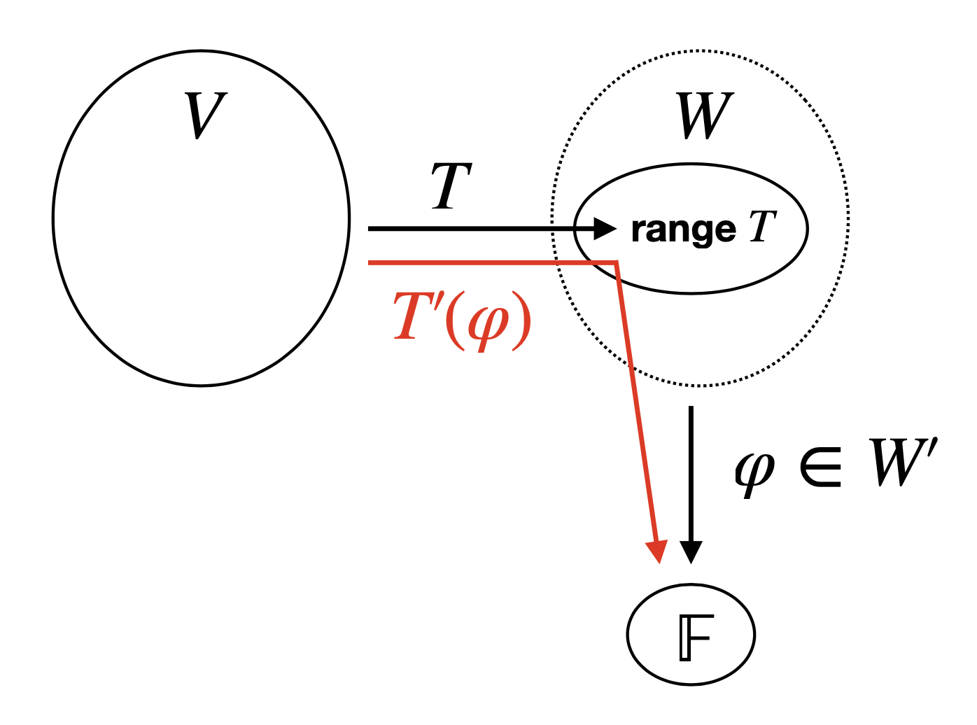
  • Can think of the action of $T’$ as piping $T$ onto $\varphi$ to accept inputs from $V$ instead of $W$. The intuition here is that, “under the hood,” $T’(\varphi)$ is using $\varphi(\range T)$ as a proxy for $T’(\varphi)(V)$.
  • If we represent the matrices of linear functionals as row vectors rather than column vectors (ie consider functionals as linear maps not vector objects), then $M(T’(\phi)) = M(\phi) \cdot M(T) = \begin{bmatrix}&\dots&\end{bmatrix} _ {1 \times m} \begin{bmatrix}&&&\\&&&\\&&&\end{bmatrix} _ {m \times n} = \begin{bmatrix}&\dots&\end{bmatrix} _ {1 \times n}.$
  • If we instead represent the matrices of linear functionals as column vectors (ie consider functionals as vector objects in vector spaces of functionals), then $M(T’(\phi)) = M(T’) \cdot M(\phi) = M(T)^T \cdot M(\phi) = \begin{bmatrix}&&&\\&&&\\&&&\end{bmatrix} _ {n \times m}\begin{bmatrix}\vdots\end{bmatrix} _ {m \times 1} = \begin{bmatrix}\vdots\end{bmatrix} _ {n \times 1}.$

• For $U \subset V$, the annihilator of $U$, denoted $U^0$, is defined by \(U^0 = \{ \varphi \in V' : \varphi(u) = 0 \text{ for all } u \in U \}\).

• $U^0$ is a subspace of $V’$.

• $\dim U + \dim U^0 = \dim V$.
  • Let $\{u_1,\dots,u_m\}$ be a basis of $U$. Extend it to a basis of $V;$ label the elements $\{u_1,\dots,u_m,u_{m+1},\dots,u_n\}$. Then the corresponding dual basis of $V’$ is $\{\varphi_1,\dots,\varphi_m,\varphi _ {m+1},\dots,\varphi_n\}$. We show $\{\varphi _ {m+1},\dots,\varphi_n\}$ is a basis of $U^0$. Linear independence is implied from construction. To see that the set spans $U^0$, consider some $\varphi \in U^0$. We need to show that $\varphi$ can be expressed as a linear combination of $\{\varphi_ { m+1},\dots,\varphi_n\}$. We know $\varphi$ is completely specified by its action on the basis vectors $\{u_1,\dots,u_m,u_{m+1},\dots,u_n\}$, and furthermore $\varphi(u_i) = 0 $ for $1 \leq i \leq m$ because $\varphi$ is an annihilator. So we need only specify the action of $\varphi$ on $\{u_{m+1},\dots,u_n\}$, which we can do by writing $\varphi = \sum_{i=m+1}^n a_i \varphi_i$ where we let $a_i = \varphi(u_i)$.
  • The intuition here is that the “dual subspace” of $V \setminus U$ contains exactly the functionals that ignore (annihilate) all the vectors in $U$.
• $\null T’ = (\range T)^0$. See dual map figure.
  • Suppose that for some $\varphi \in W’$, $(T’(\varphi))(v) = (\varphi \circ T)(v) = 0$ for all $v \in V$. This is the statement that $\varphi \circ T$ is the zero functional $\in V’$, i.e. that $\varphi \in \null T’$. When viewed as $\varphi(Tv) = 0$, this is the statement that $\varphi$ annihilates the range of $T$.
  • The connection between $T$ and $T’$ provides the dimension arithmetic for $V, W$ and that for $V’, W’$ (see below).
  • (An analogy to explain that $T’(\varphi)$ uses $\varphi(\range T)$ as a proxy for $T’(\varphi)(V)$.) Consider a set $V$ of a bunch of rich students who are trying to get into Yale, and each student $v \in V$ is in cahoots with one corrupt admissions officer $T(v)$ in the entire set $W$ of officers at Yale. Then let $\varphi \in V’$ be a function that returns the morality score of any officer such that, for any officer-in-cahoots $w \in \range T$, we have $\varphi(w) = 0$ (and presume that non-corrupt officers have some positive score). Then suppose we are interested in modifying $\varphi$ to evaluate the morality of students rather than officers. Then we could compose the two maps we have—$T$, which maps students to officers, and $\varphi$, which maps officers to scores—to get a functional $\varphi \circ T$ that maps students to morality scores using officers as a proxy. Observe that this particular functional $\varphi$ is in $\null T’$ because $T’(\varphi)$ will send every student to a score of $0$—and it is also in $(\range T)^0$ because $\varphi$ sends every officer-in-cahoots to $0$. $T’(\varphi)$ never uses moral officers in calculation because they are outside $\range T$ (see dual map figure). If we take a different functional $\psi$, say a humor score, then $\psi \circ T$ will map each student to his officer-in-cahoots’ humor score; in this case it is likely that $\psi \circ T \neq 0$, and so $\psi \notin \null T’$.
• $\rank T’ = \rank T$.
  • \[\begin{align*} \rank T' &= \dim W' - \dim \null T' \\ &= \dim W - \dim (\range T)^0 \\ &= \dim W - (\dim W - \rank T) \\ &= \rank T \end{align*}\]
• $\dim W = \dim \null T’ + \rank T$
• Remark. Given $T:V\rightarrow W$ with $M(T) = A, \dim V = n, \dim W = m, \rank T=r$, Strang’s four fundamental subspaces are:
  1. $\range T$, the column space of $A$, with dimension $r;$
  2. $\range T’$, the row space of $A$ (column space of $A^T$), with dimension $r;$
  3. $\null T$, the solutions to $Ax_n = 0$, with dimension $n-r;$
  4. $\null T’$, the solutions to $Ay_m = 0$, with dimension $m-r$.
• The matrix of $T’$ is the transpose of the matrix of $T$.
  • Consider $T: V \rightarrow W$, with $\dim V = n$ and $\dim W = m$. Let $\{v _ k\}$ and $\{w _ k\}$ be bases of $V$ and $W$, respectively, and let $A$ be the matrix representation of $T$ according to these bases. Let $C$ be the matrix representation of $T’$ according to the dual bases $\{\varphi _ k\}$ and $\{\psi _ k\}$ of $\{v _ k\}$ and $\{w _ k\}$, respectively.
  • Now consider $(T’(\psi_j))(v_k)$, where $v_k$ is a member of the basis with $1 \leq k \leq n$. Here again there are two vantage points from which to view this operation, depending on whether you use $C$ and let $v_k$ select the $k$th component from $T’(\psi_j)$, or you use $A$ and let $\psi_j$ select the $j$th component of $T(v_k)$:
    1. The dual map vantage point, with $T’$ as a linear map operating on linear functionals (which assume the role as input vectors). Then the matrix representation of $T’(\psi_j)$ is $C\psi_j,$ where $\psi_j$ is a column vector of length $m$. This returns the $j$th column of $C$, i.e. the column vector $C_{\cdot,j}$ of length $n$ representing $\sum_{r=1}^n C_{r,j}\varphi_r$, a linear functional in $V’$. The action of this linear functional on $v_k$ is to send it to the $k$th coefficient of that sum, which is $C_{k,j}$.
    2. The original map vantage point, with $T$ as a linear map operating on vectors in $V$. Then we write $(T’(\psi_j))(v_k) = \psi_j (Tv_k)$. The matrix representation of $Tv_k$ is $Av_k$, where $v_k$ is a column vector. This returns the $k$th column of $A$, i.e. the column vector $A_{\cdot, k}$ of length $m$ representing $\sum_{r=1}^m A_{r,k}w_r$, a vector in $W$. The action of $\psi_j$ on this vector is to send it to the $j$th coefficient of that sum, which is $A_{j,k}$.
  • $C _ {k,j} = A _ {j,k}$, implying $C = A^T$.
• One benefit of bra-ket notation is that, in the setting of many different types of vector spaces and maps, it clarifies the ambiguity of which map is being expressed as a matrix; which objects are assuming the role of input (column) vectors to that matrix (“kets”); and which objects are assuming the role of row vectors i.e. linear functionals (“bras”). We shall return to the topic after discussing adjoints.
  • To express $\psi_j (Tv_k)$ from the above discussion, we can write $\langle j \rvert A\lvert k\rangle$. “Ket $k$”, or $\lvert k\rangle$, is understood to be the column vector representation of $v_k$. “Bra $j$”, or $\langle j \rvert$, is understood to be the row vector representation of $\psi_j.$

Continued in part two.