Some Mathematics of Case-Control and Cohort Studies

Introduction

What do observational studies measure? What is the odds ratio? Why is it used so often, when we have measures like relative risk, which seems more intuitive?

Many educational materials geared toward the medical community are frustratingly imprecise when it comes to answering these questions, which is unfortunate given the central importance of interpreting evidence in modern medicine. Hence this primer.

Case-control vs. cohort studies

Case-control and cohort studies are two common types of observational studies, which look at the ways risk exposures correlate with disease. They stand in contrast with experimental studies, which aim to establish causality.

A case-control study compares a group of people with a given disease to a group without the disease to see if they have different rates of exposure to a risk factor. For example, suppose you want to find out if there is an association between lung cancer and smoking. A case-control study could be arranged as follows: find a group of people with lung cancer (“cases”), and a group of people without lung cancer (“controls”), and then ask all the subjects about their smoking history. These studies are so common because they are relatively inexpensive: the investigator will, by design, start with a group of subjects with the disease of interest, instead of waiting on cohorts of healthy people to develop the disease over time. However, there is a cost to the expediency of case-control studies, which is explained later.

A cohort study compares a group with a given risk exposure to a group without it to see if the disease of interest develops in the groups at different rates. So the cohort study version of the lung cancer investigation would run as follows: find a group of smokers, a group of non-smokers, and see which group develops lung cancer at a higher rate over time.¹ This is more expensive to do than a case-control study because you don’t start out with a group of subjects with the disease of interest; depending on how rare the disease is, the sample sizes have to be generally large to guarantee that the disease will show up at a significant rate. The reward for undertaking a cohort study, however, is that you can make stronger claims about the results, which will be explained below.

First, we should step back and precisely understand the mathematics of these studies.

Risk exposure and disease are correlated events under a joint probability distribution

In a given population under study, we can think of risk exposure and disease as two events $E$ and $D$ that occur with probabilities $P(E)$ and $P(D)$. That is, a subject selected at random would be exposed with probability $P(E)$ and have the disease with probability $P(D)$. Moreover, we can think of our goal as investigators to figure out all the probabilities related to $D$ and $E$, including how the events correlate. For example, we may want to know how likely a subject has a disease given that he is exposed, i.e. $P(D | E)$, which is an example of a conditional probability. Or we may want to know how the likelihood of a subject having both the disease and exposure, or $P(D, E)$, which is an example of a joint probability. In the context of joint probability distributions, $P(D)$ and $P(E)$ are called marginal probabilities because they can be calculated by summing across a row or column in a table of joint distributions and written in the margins.

Conditional and marginal probabilities can be derived if we have the joint probabilities shown in the following table.

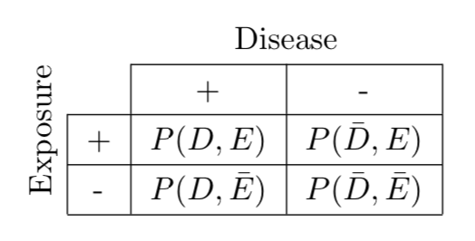
\[ \text{Figure 1. Joint probability distribution of disease } D \text{ and exposure } E \text{.} \]

As an example of a marginal probability calculation, we have $P(D) = P(D,E) + P(D,\bar{E})$, marginalizing $E$ by summing across its two outcomes. Conditional probabilities can be calculated by their definition, i.e. $P(D | E) = P(D,E)/P(E)$.

In an ideal world, we could survey the entire population perfectly (or at least have a huge random sample of the entire population) and directly calculate these joint probabilities. But this is not practical. Fortunately, we can simplify the task and still obtain some useful information.

Small observational studies allow us to estimate conditional probabilities for large populations

Whichever way you decide to sample your population, the data can be categorized in the following contingency table, where $a,b,c,d$ are the numbers of subjects that fall into the corresponding category.

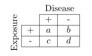
\[ \text{Figure 2. Contingency (or 2 x 2) table.} \]

However, it is crucial to understand the relationship between these numbers and the samples! The reason for this is that $a,b,c,d$ only reflect probabilities when they are divided by denominators that reflect the sizes of the study groups sampled.

If the contingency table represented a single random sample from the total population under study, then the numbers $a,b,c,d$ can each be converted to joint probabilities directly because $(a+b+c+d)$ comprises a sample, e.g. $P(D,E) = a / (a+b+c+d)$. Then we could calculate any conditional probability we would be interested in.

By contrast, case-control and cohort studies first stratify the population by $D$ or $E$, respectively, and then sample each of the two subsets. For case-control studies, we stratified the population into $D$ and $\bar{D}$, and then sampled a disease group of size $(a+c)$ and a control group of size $(b+d)$. In contrast, for cohort studies, we stratified the population into $E$ and $\bar{E}$, and sampled an exposure group of size $(a+b)$ and a non-exposure group of size $(c+d)$.

Because our samples are taken from groups conditioned on the presence (or absence) of $D$ or $E$, we can only calculate conditional probabilities; furthermore, case-control and cohort studies differ on which conditional probabilities we are allowed to calculate.

For case-control studies, we sampled one group of size $(a+c)$ from the subpopulation with disease and another of size $(b+d)$ from the subpopulation without disease, so their contingency table allows us to estimate the conditional probabilities of exposure status ($E$ or $\bar{E}$) given disease status ($D$ or $\bar{D}$). That is, for case-control studies, we can make the following estimations:

\[\begin{align} P(E | D) &= \frac{a}{a+c} \\ P(\bar{E} | D ) &= \frac{c}{a+c} \\ P(E | \bar{D}) &= \frac{b}{b+d} \\ P(\bar{E} | \bar{D} ) &= \frac{d}{b+d} \\ \label{eq:case} \end{align}\]

For cohort studies, we sampled one group of size $(a+b)$ from the exposure subpopulation, and another of size $(c + d)$ from the non-exposure subpopulation, so their contingency table reflects the conditional probability of disease status given exposure status. That is, for cohort studies, we can make the following estimations:

\[\begin{align} P(D | E) &= \frac{a}{a+b} \\ P(\bar{D} | E ) &= \frac{b}{a+b} \\ P(D | \bar{E}) &= \frac{c}{c+d} \\ P(\bar{D} | \bar{E} ) &= \frac{d}{c+d} \\ \label{eq:cohort} \end{align}\]

Relative risk

In cohort studies, we can now define the relative risk (RR) as the ratio of the rate of disease in the exposed group to that of the non-exposed group, or

\[\begin{equation} RR := \frac{P(D|E)}{P(D|\bar{E})} = \frac{a/(a+b)}{c/(c+d)}, \label{eq:rr1} \end{equation}\]

which simplifies to $\frac{a(c+d)}{c(a+b)}$.

RR is very intuitive. An RR of 3 means that subjects in the exposed group had the disease at 3 times the rate as subjects in the non-exposed group.

We are not allowed to use RR in case-control studies because in such studies we cannot estimate $P(D|E)$ or $P(D|\bar{E})$; we selected groups based on disease status to compare rates of exposure, so we are unable to make claims about rates of disease based on exposure status.

The symmetry of the odds ratio allows it to be calculated from either study

In statistics, odds are an expression of relative probabilities. The odds for an event $A$ (or the odds “of” $A$) can be defined as $P(A)/P(\bar{A})$. For example, if the odds for $A$ are 4 to 1 (or simply 4), then for every 4 events there is 1 non-event. Contrast this with probability; in our example we have $P(A)=4/5$. It should be clear by now that odds are not synonymous with “chance” or “probability”! Probabilities range from 0 to 1; odds range from 0 to $\infty$.

Odds have a useful property of being invertible. The odds against $A$ are simply the reciprocal of the odds for $A$. In our example, it would be 1/4. Compare this to $P(\bar{A})$, which is $1 - P(A)$; this expression is less nice to work with.

The odds ratio comes into play when looking at the association between two events, say our two events $D$ and $E$. Going by its name, it is equivalent to the ratio of the odds of $D$ in the presence of $E$ and the odds of $D$ in the absence of $E$.

\[\begin{equation} OR = \frac{P(D|E)/P(\bar{D}|E)}{P(D|\bar{E})/P(\bar{D}|\bar{E})} \label{eq:orcohort} \end{equation}\]

The OR looks like it depends on probabilities conditional on $E$. But fortunately, it is symmetric and can be expressed as probabilities conditional on $D$:

\[\begin{equation} OR = \frac{P(E|D)/P(\bar{E}|D)}{P(E|\bar{D})/P(\bar{E}|\bar{D})} \label{eq:orcc} \end{equation}\]

This is because the OR is really a symmetric expression of the joint probabilities we so wanted to estimate in the first place! Starting from $\eqref{eq:orcohort}$, we have

\[\begin{align} \require{cancel} \frac{P(D|E)/P(\bar{D}|E)}{P(D|\bar{E})/P(\bar{D}|\bar{E})} &= \frac{ \left(\frac{P(D,E)}{P(E)}\right) / P(\bar{D}|E) }{ \left(\frac{P(D,\bar{E})}{P(\bar{E})}\right) / P(\bar{D}|\bar{E})} \\ \nonumber \\ &= \frac{ \left(\frac{P(D,E)}{\cancel{P(E)}}\right) / \left(\frac{P(\bar{D}, E)}{\cancel{P(E)}}\right) }{ \left(\frac{P(D,\bar{E})}{\cancel{P(\bar{E})}}\right) / \left(\frac{P(\bar{D},\bar{E})}{\cancel{P(\bar{E})}}\right) } \\ \nonumber \\ &= \frac{ P(D,E) / P(\bar{D}, E) }{ P(D,\bar{E}) / P(\bar{D},\bar{E}) } \\ \nonumber \\ &= \frac{ P(D,E) P(\bar{D},\bar{E}) }{ P(\bar{D},E) P(D,\bar{E}) } \end{align}\]

Amazingly, the OR turns out to be this beautiful symmetric expression of the joint probabilities.

Calculating odds ratios from contingency tables

Because the OR can be calculated with probabilities conditional on $D$ or $E$, we can calculate it from either case-control or cohort studies. For case-control studies, we plug $a,b,c,d$ into $\eqref{eq:orcc}$, which expressed OR in terms of probabilities conditioned on $D$. We get the ratio of the odds of exposure in the diseased group to that of the non-diseased group, or

\[\begin{equation} \frac{(a/c)}{(b/d)}, \label{eq:or1} \end{equation}\]

which simplifies to $ad/bc$.

For cohort studies, we plug $a,b,c,d$ into $\eqref{eq:orcohort}$, which expressed OR in terms of probabilities conditioned on $E$. We get the ratio of the odds of disease in the exposed group to that of the non-exposed group, or

\[\begin{equation} \frac{(a/b)}{(c/d)}, \label{eq:or2} \end{equation}\]

which also simplifies to $ad/bc$.

Deception in lazy textbooks

Here are two common areas of bad teaching that should be clarified explicitly.

Properly interpreting the definition of ORs

Because $\eqref{eq:or2}$ is arithmetically equivalent to $\eqref{eq:or1}$, we can mindlessly calculate OR the same way regardless of whether the contingency table came from a cohort or case-control study. However, it is important to interpret this convenience correctly! For example, many textbooks will define OR as $\eqref{eq:or2}$, which gives the impression that $(a/b)$ and $(c/d)$ always give the odds of disease given exposure status; but this interpretation is accurate only in cohort studies (where you have $P(D|E)$ and $P(D|\bar{E})$) and incorrect in the context of case-control studies (where you do not)! For case-control studies, the terms $(a/b)$ and $(c/d)$ are meaningless and do not reflect odds because $a$ and $b$ are taken from different samples (and likewise for $c$ and $d$); it is a sheer coincidence that taking their ratio is arithmetically equivalent to the ratio of $(a/c)$ and $(b/d)$, which are the only odds you can calculate. In that case you should think in terms of $\eqref{eq:or1}$ with the understanding that you’re calculating OR from $P(E|D)$ and $P(E|\bar{D})$. Do not be mislead into thinking your contingency table contains more information than it actually does.

Why OR approximates RR when the disease is rare

The odds ratio is an approximation of RR when the incidence of disease is low (i.e., the disease is rare). The “proof” of this also should be properly understood. Assuming a contingency table derived from a cohort study, if $a \ll b$ and $c \ll d$, then we have

\[\begin{equation} RR = \frac{P(D|E)}{P(D|\bar{E})} = \frac{a/(a+b)}{c/(c+d)} \approx \frac{a/b}{c/d} = OR. \end{equation}\]

However, this explanation is nonsensical if $a,b,c,d$ come from a case-control study’s contingency table, because in that case $RR \neq \frac{a/(a+b)}{c/(c+d)}$! But case-control studies are where this approximation must be used, and various resources give this false explanation.

The precise explanation is that, when the disease is rare,

\[\begin{equation} P(D|E) \approx \text{Odds of } D \text{ given } E, \end{equation}\]

and

\[\begin{equation} P(D | \bar{E}) \approx \text{Odds of } D \text{ given } \bar{E}. \end{equation}\]

So, finally, we have

\[\begin{equation} RR = \frac{P(D|E)}{P(D|\bar{E})} \approx \frac{\text{Odds of } D \text{ given } E}{\text{Odds of } D \text{ given } \bar{E}} = OR, \end{equation}\]

which we can calculate from

\[\begin{equation} \frac{\text{Odds of } E \text{ given } D}{\text{Odds of } E \text{ given } \bar{D}} = \frac{(a/c)}{(b/d)}. \end{equation}\]

---